
Titik berat pada bidang studi ini adalah mempelajari bagaimana cara-cara mendesain suatu peralatan mesin yang berpangkal pada mata kuliah – mata kuliah Kinematika, Dinamika, Mekanika Teknik, Elemen Mesin yang menerapkannya pada mata kuliah – mata kuliah Pesawat pengangkat, Getaran, Mekanika teknik Lanjut, Analisa tegangan Eksperimen, Mekanika Getaran dan Struktur, Metode Elemen Hingga, Stabilitas kendaraan dan sebagainya.
KINEMATICS
It is natural to begin this discussion by considering the various possible types of motion in themselves, leaving out of account for a time the causes to which the initiation of motion may be ascribed; this preliminary enquiry constitutes the science of Kinematics.
—ET Whittaker.
Kinematics is the branch of classical mechanics that describes the motion of bodies (objects) and systems (groups of objects) without consideration of the forces that cause the motion.
Kinematics is not to be confused with another branch of classical mechanics: analytical dynamics (the study of the relationship between the motion of objects and its causes), sometimes subdivided into kinetics (the study of the relation between external forces and motion) and statics (the study of the relations in a system at equilibrium). Kinematics also differs from dynamics as used in modern-day physics to describe time-evolution of a system. The term kinematics is less common today than in the past, but still has a role in physics. (See analytical dynamics for more detail on usage). The term kinematics also finds use in biomechanics and animal locomotion.
The simplest application of kinematics is for particle motion, translational or rotational. The next level of complexity comes from the introduction of rigid bodies, which are collections of particles having time invariant distances between themselves. Rigid bodies might undergo translation and rotation or a combination of both. A more complicated case is the kinematics of a system of rigid bodies, which may be linked together by mechanical joints. Kinematics can be used to find the possible range of motion for a given mechanism, or, working in reverse, can be used to design a mechanism that has a desired range of motion. The movement of a crane and the oscillations of a piston in an engine are both simple kinematic systems. The crane is a type of open kinematic chain, while the piston is part of a closed four-bar linkage.
This article describes a particle in planar motion when observed from non-inertial reference frames. The most famous examples of planar motion are related to the motion of two spheres that are gravitationally attracted to one another, and the generalization of this problem to planetary motion. See centrifugal force, two-body problem, orbit and Kepler's laws of planetary motion. Those problems fall in the general field of analytical dynamics, the determination of orbits from given laws of force. This article is focused more on the kinematical issues surrounding planar motion, that is, determination of the forces necessary to result in a certain trajectory given the particle trajectory. General results presented in fictitious forces here are applied to observations of a moving particle as seen from several specific non-inertial frames, for example, a local frame (one tied to the moving particle so it appears stationary), and a co-rotating frame (one with an arbitrarily located but fixed axis and a rate of rotation that makes the particle appear to have only radial motion and zero azimuthal motion). The Lagrangian approach to fictitious forces is introduced.
Unlike real forces such as electromagnetic forces, fictitious forces do not originate from physical interactions between objects.
Analysis using fictitious forces
Kinematics is not to be confused with another branch of classical mechanics: analytical dynamics (the study of the relationship between the motion of objects and its causes), sometimes subdivided into kinetics (the study of the relation between external forces and motion) and statics (the study of the relations in a system at equilibrium). Kinematics also differs from dynamics as used in modern-day physics to describe time-evolution of a system. The term kinematics is less common today than in the past, but still has a role in physics. (See analytical dynamics for more detail on usage). The term kinematics also finds use in biomechanics and animal locomotion.
The simplest application of kinematics is for particle motion, translational or rotational. The next level of complexity comes from the introduction of rigid bodies, which are collections of particles having time invariant distances between themselves. Rigid bodies might undergo translation and rotation or a combination of both. A more complicated case is the kinematics of a system of rigid bodies, which may be linked together by mechanical joints. Kinematics can be used to find the possible range of motion for a given mechanism, or, working in reverse, can be used to design a mechanism that has a desired range of motion. The movement of a crane and the oscillations of a piston in an engine are both simple kinematic systems. The crane is a type of open kinematic chain, while the piston is part of a closed four-bar linkage.
Mechanics of planar particle motion
This article describes a particle in planar motion when observed from non-inertial reference frames. The most famous examples of planar motion are related to the motion of two spheres that are gravitationally attracted to one another, and the generalization of this problem to planetary motion. See centrifugal force, two-body problem, orbit and Kepler's laws of planetary motion. Those problems fall in the general field of analytical dynamics, the determination of orbits from given laws of force. This article is focused more on the kinematical issues surrounding planar motion, that is, determination of the forces necessary to result in a certain trajectory given the particle trajectory. General results presented in fictitious forces here are applied to observations of a moving particle as seen from several specific non-inertial frames, for example, a local frame (one tied to the moving particle so it appears stationary), and a co-rotating frame (one with an arbitrarily located but fixed axis and a rate of rotation that makes the particle appear to have only radial motion and zero azimuthal motion). The Lagrangian approach to fictitious forces is introduced.
Unlike real forces such as electromagnetic forces, fictitious forces do not originate from physical interactions between objects.
Analysis using fictitious forces
The appearance of fictitious forces normally is associated with use of a non-inertial frame of reference, and their absence with use of an inertial frame of reference. The connection between inertial frames and fictitious forces (also called inertial forces or pseudo-forces), is expressed, for example, by Arnol'd:
The equations of motion in an non-inertial system differ from the equations in an inertial system by additional terms called inertial forces. This allows us to detect experimentally the non-inertial nature of a system.A slightly different tack on the subject is provided by Iro:
– V. I. Arnol'd: Mathematical Methods of Classical Mechanics Second Edition, p. 129
An additional force due to nonuniform relative motion of two reference frames is called a pseudo-force.
– H Iro in A Modern Approach to Classical Mechanics p. 180
Fictitious forces do not appear in the equations of motion in an inertial frame of reference: in an inertial frame, the motion of an object is explained by the real impressed forces. In a non-inertial frame such as a rotating frame, however, Newton's first and second laws still can be used to make accurate physical predictions provided fictitious forces are included along with the real forces. For solving problems of mechanics in non-inertial reference frames, the advice given in textbooks is to treat the fictitious forces like real forces and to pretend you are in an inertial frame.
Treat the fictitious forces like real forces, and pretend you are in an inertial frame.It should be mentioned that "treating the fictitious forces like real forces" means, in particular, that fictitious forces as seen in a particular non-inertial frame transform as vectors under coordinate transformations made within that frame, that is, like real forces.
– Louis N. Hand, Janet D. Finch Analytical Mechanics, p. 267
Moving objects and observational frames of reference
Next, it is observed that time varying coordinates are used in both inertial and non-inertial frames of reference, so the use of time varying coordinates should not be confounded with a change of observer, but is only a change of the observer's choice of description. Elaboration of this point and some citations on the subject follow.
Frame of reference and coordinate system
The term frame of reference is used often in a very broad sense, but for the present discussion its meaning is restricted to refer to an observer's state of motion, that is, to either an inertial frame of reference or a non-inertial frame of reference.
The term coordinate system is used to differentiate between different possible choices for a set of variables to describe motion, choices available to any observer, regardless of their state of motion. Examples are Cartesian coordinates, polar coordinates and (more generally) curvilinear coordinates.
Here are two quotes relating "state of motion" and "coordinate system":
We first introduce the notion of reference frame, itself related to the idea of observer: the reference frame is, in some sense, the "Euclidean space carried by the observer". Let us give a more mathematical definition:… the reference frame is... the set of all points in the Euclidean space with the rigid body motion of the observer. The frame, denoted, is said to move with the observer.… The spatial positions of particles are labelled relative to a frame
– Jean Salençon, Stephen Lyle. (2001). Handbook of Continuum Mechanics: General Concepts, Thermoelasticity p. 9
In traditional developments of special and general relativity it has been customary not to distinguish between two quite distinct ideas. The first is the notion of a coordinate system, understood simply as the smooth, invertible assignment of four numbers to events in spacetime neighborhoods. The second, the frame of reference, refers to an idealized system used to assign such numbers … To avoid unnecessary restrictions, we can divorce this arrangement from metrical notions. … Of special importance for our purposes is that each frame of reference has a definite state of motion at each event of spacetime.…Within the context of special relativity and as long as we restrict ourselves to frames of reference in inertial motion, then little of importance depends on the difference between an inertial frame of reference and the inertial coordinate system it induces. This comfortable circumstance ceases immediately once we begin to consider frames of reference in nonuniform motion even within special relativity.…the notion of frame of reference has reappeared as a structure distinct from a coordinate system.
– John D. Norton: General Covariance and the Foundations of General Relativity: eight decades of dispute, Rep. Prog. Phys., 56, pp. 835-7.
Time varying coordinate systems
In a general coordinate system, the basis vectors for the coordinates may vary in time at fixed positions, or they may vary with position at fixed times, or both. It may be noted that coordinate systems attached to both inertial frames and non-inertial frames can have basis vectors that vary in time, space or both, for example the description of a trajectory in polar coordinates as seen from an inertial frame. or as seen from a rotating frame. A time-dependent description of observations does not change the frame of reference in which the observations are made and recorded.
Fictitious forces in a local coordinate system
 |
| Figure 1: Local coordinate system for planar motion on a curve. Two different positions are shown for distances s and s + ds along the curve. At each position s, unit vector un points along the outward normal to the curve and unit vector ut is tangential to the path. The radius of curvature of the path is ρ as found from the rate of rotation of the tangent to the curve with respect to arc length, and is the radius of the osculating circle at position s. The unit circle on the left shows the rotation of the unit vectors with s. |
 |
| The arc length s(t) measures distance along the skywriter's trail |
In discussion of a particle moving in a circular orbit, in an inertial frame of reference one can identify the centripetal and tangential forces. It then seems to be no problem to switch hats, change perspective, and talk about the fictitious forces commonly called the centrifugal and Euler force. But what underlies this switch in vocabulary is a change of observational frame of reference from the inertial frame where we started, where centripetal and tangential forces make sense, to a rotating frame of reference where the particle appears motionless and fictitious centrifugal and Euler forces have to be brought into play. That switch is unconscious, but real.
Suppose we sit on a particle in general planar motion (not just a circular orbit). What analysis underlies a switch of hats to introduce fictitious centrifugal and Euler forces?
To explore that question, begin in an inertial frame of reference. By using a coordinate system commonly used in planar motion, the so-called local coordinate system, as shown in Figure 1, it becomes easy to identify formulas for the centripetal inward force normal to the trajectory (in direction opposite to un in Figure 1), and the tangential force parallel to the trajectory (in direction ut), as shown next.
To introduce the unit vectors of the local coordinate system shown in Figure 1, one approach is to begin in Cartesian coordinates in an inertial framework and describe the local coordinates in terms of these Cartesian coordinates. In Figure 1, the arc length s is the distance the particle has traveled along its path in time t. The path r (t) with components x(t), y(t) in Cartesian coordinates is described using arc length s(t) as:
![\mathbf{r}(s) = \left[ x(s),\ y(s) \right] \ .](http://upload.wikimedia.org/math/b/1/e/b1eeb9960e429ffc4a2e19623c698bd8.png)
One way to look at the use of s is to think of the path of the particle as sitting in space, like the trail left by a skywriter, independent of time. Any position on this path is described by stating its distance s from some starting point on the path. Then an incremental displacement along the path ds is described by:
As an aside, notice that the use of unit vectors that are not aligned along the Cartesian xy-axes does not mean we are no longer in an inertial frame. All it means is that we are using unit vectors that vary with s to describe the path, but still observe the motion from the inertial frame.
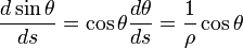
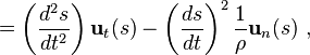
Using the tangent vector, the angle of the tangent to the curve, say θ, is given by:
Using the above results for the path properties in terms of s, the acceleration in the inertial reference frame as described in terms of the components normal and tangential to the path of the particle can be found in terms of the function s(t) and its various time derivatives (as before, primes indicate differentiation with respect to s):
Next, we change observational frames. Sitting on the particle, we adopt a non-inertial frame where the particle is at rest (zero velocity). This frame has a continuously changing origin, which at time t is the center of curvature (the center of the osculating circle in Figure 1) of the path at time t, and whose rate of rotation is the angular rate of motion of the particle about that origin at time t. This non-inertial frame also employs unit vectors normal to the trajectory and parallel to it.
The angular velocity of this frame is the angular velocity of the particle about the center of curvature at time t. The centripetal force of the inertial frame is interpreted in the non-inertial frame where the body is at rest as a force necessary to overcome the centrifugal force. Likewise, the force causing any acceleration of speed along the path seen in the inertial frame becomes the force necessary to overcome the Euler force in the non-inertial frame where the particle is at rest. There is zero Coriolis force in the frame, because the particle has zero velocity in this frame. For a pilot in an airplane, for example, these fictitious forces are a matter of direct experience. However, these fictitious forces cannot be related to a simple observational frame of reference other than the particle itself, unless it is in a particularly simple path, like a circle.
That said, from a qualitative standpoint, the path of an airplane can be approximated by an arc of a circle for a limited time, and for the limited time a particular radius of curvature applies, the centrifugal and Euler forces can be analyzed on the basis of circular motion with that radius. See article discussing turning an airplane.
Next, reference frames rotating about a fixed axis are discussed in more detail.
![d\mathbf{r}(s) = \left[ dx(s),\ dy(s) \right]=\left[ x'(s),\ y'(s) \right] ds \ ,](http://upload.wikimedia.org/math/5/4/e/54e45e44e7404b9ea347f402f1764d0f.png)
![\left[ x'(s)^2 + y'(s)^2 \right] = 1 \ .](http://upload.wikimedia.org/math/6/3/9/639e16921e9aa65952053c44c8049bd1.png) (Eq. 1)
(Eq. 1)
![\mathbf{u}_t(s) = \left[ x'(s), \ y'(s) \right] \ ,](http://upload.wikimedia.org/math/a/9/2/a923437f5e9ddb98da70bbb1088314bc.png)
![\mathbf{u}_n(s) = \left[ y'(s),\ -x'(s) \right] \ ,](http://upload.wikimedia.org/math/3/0/e/30e4981e3cbbb1022b5e0207ebb23366.png)
As an aside, notice that the use of unit vectors that are not aligned along the Cartesian xy-axes does not mean we are no longer in an inertial frame. All it means is that we are using unit vectors that vary with s to describe the path, but still observe the motion from the inertial frame.
Using the tangent vector, the angle of the tangent to the curve, say θ, is given by:
 and
and 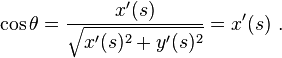


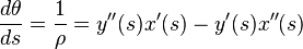


Using the above results for the path properties in terms of s, the acceleration in the inertial reference frame as described in terms of the components normal and tangential to the path of the particle can be found in terms of the function s(t) and its various time derivatives (as before, primes indicate differentiation with respect to s):

![= \frac{d}{dt}\left[\frac{ds}{dt} \left( x'(s), \ y'(s) \right) \right]\](http://upload.wikimedia.org/math/b/8/4/b840800b347d0546f05a2dec9819a24a.png)

Next, we change observational frames. Sitting on the particle, we adopt a non-inertial frame where the particle is at rest (zero velocity). This frame has a continuously changing origin, which at time t is the center of curvature (the center of the osculating circle in Figure 1) of the path at time t, and whose rate of rotation is the angular rate of motion of the particle about that origin at time t. This non-inertial frame also employs unit vectors normal to the trajectory and parallel to it.
The angular velocity of this frame is the angular velocity of the particle about the center of curvature at time t. The centripetal force of the inertial frame is interpreted in the non-inertial frame where the body is at rest as a force necessary to overcome the centrifugal force. Likewise, the force causing any acceleration of speed along the path seen in the inertial frame becomes the force necessary to overcome the Euler force in the non-inertial frame where the particle is at rest. There is zero Coriolis force in the frame, because the particle has zero velocity in this frame. For a pilot in an airplane, for example, these fictitious forces are a matter of direct experience. However, these fictitious forces cannot be related to a simple observational frame of reference other than the particle itself, unless it is in a particularly simple path, like a circle.
That said, from a qualitative standpoint, the path of an airplane can be approximated by an arc of a circle for a limited time, and for the limited time a particular radius of curvature applies, the centrifugal and Euler forces can be analyzed on the basis of circular motion with that radius. See article discussing turning an airplane.
Next, reference frames rotating about a fixed axis are discussed in more detail.
Fictitious forces in polar coordinates
Description of particle motion often is simpler in non-Cartesian coordinate systems, for example, polar coordinates. When equations of motion are expressed in terms of any curvilinear coordinate system, extra terms appear that represent how the basis vectors change as the coordinates change. These terms arise automatically on transformation to polar (or cylindrical) coordinates and are thus not fictitious forces, but rather are simply added terms in the acceleration in polar coordinates.
Assuming it is clear that "state of motion" and "coordinate system" are different, it follows that the dependence of centrifugal force (as in this article) upon "state of motion" and its independence from "coordinate system", which contrasts with the "coordinate" version with exactly the opposite dependencies, indicates that two different ideas are referred to by the terminology "fictitious force". The present article emphasizes one of these two ideas ("state-of-motion"), although the other also is described.
Below, polar coordinates are introduced for use in (first) an inertial frame of reference and then (second) in a rotating frame of reference. The two different uses of the term "fictitious force" are pointed out. First, however, follows a brief digression to explain further how the "coordinate" terminology for fictitious force has arisen.
In classical mechanics, the Lagrangian is defined as the kinetic energy, T, of the system minus its potential energy, U. In symbols,
Here are some definitions:
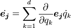
To proceed, consider a single particle, and introduce the generalized coordinates as {qk} = (r, θ). Then Hildebrand shows in polar coordinates with the qk = (r, θ) the "generalized momenta" are:
 Careful reading of Hildebrand shows he doesn't discuss the role of "inertial frames of reference", and in fact, says "[The] presence or absence [of inertia forces] depends, not upon the particular problem at hand but upon the coordinate system chosen." By coordinate system presumably is meant the choice of {qk}. Later he says "If accelerations associated with generalized coordinates are to be of prime interest (as is usually the case), the [nonaccelerational] terms may be conveniently transferred to the right … and considered as additional (generalized) inertia forces. Such inertia forces are often said to be of the Coriolis type."
In short, the emphasis of some authors upon coordinates and their derivatives and their introduction of (generalized) fictitious forces that do not vanish in inertial frames of reference is an outgrowth of the use of generalized coordinates in Lagrangian mechanics. For example, see McQuarrie. Hildebrand, and von Schwerin.Below is an example of this usage as employed in the design of robotic manipulators:
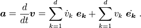
For a robot manipulator, the equations may be written in a form using Christoffel symbols Γijk (discussed further below) as:
The introduction of generalized fictitious forces often is done without notification and without specifying the word "generalized". This sloppy use of terminology leads to endless confusion because these generalized fictitious forces, unlike the standard "state-of-motion" fictitious forces, do not vanish in inertial frames of reference.
In an inertial frame, let be the position vector of a moving particle. Its Cartesian components (x, y) are:
Unit vectors are defined in the radially outward direction:
:
 , in an inertial frame of reference Newton's second law expressed in polar coordinates is:
From a mathematical standpoint, however, it sometimes is handy to put only the second-order derivatives on the right side of this equation; that is we write the above equation by rearrangement of terms as:
These newly defined "forces" are non-zero in an inertial frame, and so certainly are not the same as the previously identified fictitious forces that are zero in an inertial frame and non-zero only in a non-inertial frame. In this article, these newly defined forces are called the "coordinate" centrifugal force and the "coordinate" Coriolis force to separate them from the "state-of-motion" forces.
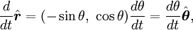
Here is an illustration showing the so called "centrifugal term"  does not transform as a true force, putting any reference to this term not just as a "term", but as a centrifugal force, in a dubious light. Suppose in frame S a particle moves radially away from the origin at a constant velocity. See Figure 2. The force on the particle is zero by Newton's first law. Now we look at the same thing from frame S' , which is the same, but displaced in origin. In S' the particle still is in straight line motion at constant speed, so again the force is zero.
What if we use polar coordinates in the two frames? In frame S the radial motion is constant and there is no angular motion. Hence, the acceleration is:
 and
and  . There is no force, including no "force" in frame S. In frame S' , however, we have:
 nor
nor  is zero. That is, we cannot obtain zero force (zero
  ) if we retain only
  as the acceleration; we need both terms.
Despite the above facts, suppose we adopt polar coordinates, and wish to say that is "centrifugal force", and reinterpret  as "acceleration" (without dwelling upon any possible justification). How does this decision fare when we consider that a proper formulation of physics is geometry and coordinate-independent? See the article on general covariance. To attempt to form a covariant expression, this so-called centrifugal "force" can be put into vector notation as:
 a unit vector normal to the plane of motion. Unfortunately, although this expression formally looks like a vector, when an observer changes origin the value of
  changes (see Figure 2), so observers in the same frame of reference standing on different street corners see different "forces" even though the actual events they witness are identical. How can a physical force (be it fictitious or real) be zero in one frame S, but non-zero in another frame S' identical, but a few feet away? Even for exactly the same particle behavior the expression is different in every frame of reference, even for very trivial distinctions between frames. In short, if we take as "centrifugal force", it does not have a universal significance: it is unphysical.
Beyond this problem, the real impressed net force is zero. (There is no real impressed force in straight-line motion at constant speed). If we adopt polar coordinates, and wish to say that is "centrifugal force", and reinterpret as "acceleration", the oddity results in frame S' that straight-line motion at constant speed requires a net force in polar coordinates, but not in Cartesian coordinates. Moreover, this perplexity applies in frame S', but not in frame S.
The absurdity of the behavior of indicates that one must say that is not centrifugal force, but simply one of two terms in the acceleration. This view, that the acceleration is composed of two terms, is frame-independent: there is zero centrifugal force in any and every inertial frame. It also is coordinate-system independent: we can use Cartesian, polar, or any other curvilinear system: they all produce zero.
Apart from the above physical arguments, of course, the derivation above, based upon application of the mathematical rules of differentiation, shows the radial acceleration does indeed consist of the two terms .
.
That said, the next subsection shows there is a connection between these centrifugal and Coriolis terms and the fictitious forces that pertain to a particular rotating frame of reference (as distinct from an inertial frame).
In the case of planar motion of a particle, the "coordinate" centrifugal and Coriolis acceleration terms found above to be non-zero in an inertial frame can be shown to be the negatives of the "state-of-motion" centrifugal and Coriolis terms that appear in a very particular non-inertial co-rotating frame (see next subsection). See Figure 3. To define a co-rotating frame, first an origin is selected from which the distance r(t) to the particle is defined. An axis of rotation is set up that is perpendicular to the plane of motion of the particle, and passing through this origin. Then, at the selected moment t, the rate of rotation of the co-rotating frame Ω is made to match the rate of rotation of the particle about this axis, dθ/dt. The co-rotating frame applies only for a moment, and must be continuously re-selected as the particle moves. For more detail, see Polar coordinates, centrifugal and Coriolis terms.
 is the radial component of the Coriolis force per unit mass, where
  is the tangential component of the particle velocity as seen in the rotating frame. The term
  is the so-called azimuthal component of the Coriolis force per unit mass. In fact, these extra terms can be used to measure Ω and provide a test to see whether or not the frame is rotating, just as explained in the example of rotating identical spheres. If the particle's motion can be described by the observer using Newton's laws of motion without these Ω-dependent terms, the observer is in an inertial frame of reference where Ω=0.
These "extra terms" in the acceleration of the particle are the "state of motion" fictitious forces for this rotating frame, the forces introduced by rotation of the frame at angular rate Ω.
In this rotating frame, what are the "coordinate" fictitious forces? As before, suppose we choose to put only the second-order time derivatives on the right side of Newton's law:
 as some so-called "acceleration", then the terms
 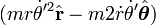 are added to the so-called "fictitious force", which are not "state-of-motion" fictitious forces, but are actually components of force that persist even when Ω=0, that is, they persist even in an inertial frame of reference. Because these extra terms are added, the "coordinate" fictitious force is not the same as the "state-of-motion" fictitious force. Because of these extra terms, the "coordinate" fictitious force is not zero even in an inertial frame of reference.
To quote Bullo and Lewis: "Only in exceptional circumstances can the configuration of Lagrangian system be described by a vector in a vector space. In the natural mathematical setting, the system's configuration space is described loosely as a curved space, or more accurately as a differentiable manifold."
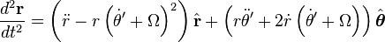
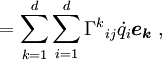
Instead of Cartesian coordinates, when equations of motion are expressed in a curvilinear coordinate system, Christoffel symbols appear in the acceleration of a particle expressed in this coordinate system, as described below in more detail. Consider description of a particle motion from the viewpoint of an inertial frame of reference in curvilinear coordinates. Suppose the position of a point P in Cartesian coordinates is (x, y, z) and in curvilinear coordinates is (q1, q2. q3). Then functions exist that relate these descriptions:
Using relations like this one,
"State-of-motion" versus "coordinate" fictitious forces
Earlier in this article a distinction was introduced between two terminologies, the fictitious forces that vanish in an inertial frame of reference are called in this article the "state-of-motion" fictitious forces and those that originate from differentiation in a particular coordinate system are called "coordinate" fictitious forces. Using the expression for the acceleration above, Newton's law of motion in the inertial frame of reference becomes:
The "coordinate" approach to Newton's law above is to retain the second-order time derivatives of the coordinates {qk} as the only terms on the right side of this equation, motivated more by mathematical convenience than by physics. To that end, the force law can be rewritten, taking the second summation to the force-side of the equation as:
is now:
If the frame is not inertial, for example, in a rotating frame of reference, the "state-of-motion" fictitious forces are included in the above "coordinate" fictitious force expression. Also, if the "acceleration" expressed in terms of first-order time derivatives of the velocity happens to result in terms that are not simply second-order derivatives of the coordinates {qk} in time, then these terms that are not second-order also are brought to the force-side of the equation and included with the fictitious forces. From the standpoint of a Lagrangian formulation, they can be called generalized fictitious forces. See Hildebrand , for example.
Formulation of dynamics in terms of Christoffel symbols and the "coordinate" version of fictitious forces is used often in the design of robots in connection with a Lagrangian formulation of the equations of motion.
Particle kinematics is the study of the kinematics of a single particle. The results obtained in particle kinematics are used to study the kinematics of collection of particles, dynamics and in many other branches of mechanics.
Position is usually described by mathematical quantities that have all these three attributes: the most common are vectors and complex numbers. Usually, only vectors are used. For measurement of distances and directions, usually three dimensional coordinate systems are used with the origin coinciding with the reference point. A three-dimensional coordinate system (whose origin coincides with the reference point) with some provision for time measurement is called a reference frame or frame of reference or simply frame. All observations in physics are incomplete without the reference frame being specified.
Distance
In physics,distance can be defined as when a particle start moving one place to another place and complete his journey at the intial pont is said distance for example -if a body start its journey at point A and follow the path B AND C and at last it came on its intial point A then it is called distance. It is a scalar quantity, describing the length of the path between two points along which the particle has traveled.
When considering the motion of a particle over time, distance is the length of the particle's path and may be different from displacement, which is the change from its initial position to its final position. For example, a race car traversing a 10 km closed loop from start to finish travels a distance of 10 km; its displacement, however, is zero because it arrives back at its initial position.
If the position of the particle is known as a function of time (r = r(t)), the distance s it travels from time t1 to time t2 can be found by
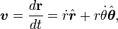
Velocity is the measure of the rate of change in position with respect to time, that is, how the distance of a point changes with each instant of time. Velocity also is a vector. Instantaneous velocity (the velocity at an instant of time) can be defined as the limiting value of average velocity as the time interval Δt becomes smaller and smaller. Both Δr and Δt approach zero but the ratio v approaches a non-zero limit v. That is,
As a position vector itself is frame dependent, velocity is also dependent on the reference frame.
The speed of an object is the magnitude |v| of its velocity. It is a scalar quantity:
Acceleration is the vector quantity describing the rate of change with time of velocity. Instantaneous acceleration (the acceleration at an instant of time) is defined as the limiting value of average acceleration as Δt becomes smaller and smaller. Under such a limit, a → a.
If the acceleration is non-zero but constant, the motion is said to be motion with constant acceleration. On the other hand, if the acceleration is variable, the motion is called motion with variable acceleration. In motion with variable acceleration, the rate of change of acceleration is called the jerk.
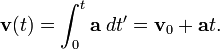
Integrating acceleration a with respect to time t gives the change in velocity. When acceleration is constant both in direction and in magnitude, the point is said to be undergoing uniformly accelerated motion. In this case, the integral relations can be simplified:
A relationship without explicit time dependence may also be derived for one-dimensional motion. Noting that at = v − v0,
For example, let Ann move with velocity relative to the reference (we drop the O subscript for convenience) and let Bob move with velocity
  , each velocity given with respect to the ground (point O). To find how fast Ann is moving relative to Bob (we call this velocity
  ), the equation above gives:
we simply rearrange this equation to obtain:
Consider an object that is fired directly upwards and falls back to the ground so that its trajectory is contained in a straight line. If we adopt the convention that the upward direction is the positive direction, the object experiences a constant acceleration of approximately −9.81 m s−2. Therefore, its motion can be modeled with the equations governing uniformly accelerated motion.
For the sake of example, assume the object has an initial velocity of +50 m s−1. There are several interesting kinematic questions we can ask about the particle's motion:
Suppose that an object is not fired vertically but is fired at an angle θ from the ground. The object will then follow a parabolic trajectory, and its horizontal motion can be modeled independently of its vertical motion. Assume that the object is fired at an initial velocity of 50 m s−1 and 30° from the horizontal.
Kinematics is the study of how things move. Here, we are interested in the motion of normal objects in our world. A normal object is visible, has edges, and has a location that can be expressed with (x, y, z) coordinates. We will not be discussing the motion of atomic particles or black holes or light.
We will create a vocabulary and a group of mathematical methods that will describe this ordinary motion. Understand that we will be developing a language for describing motion only. We won't be concerned with what is causing or changing the motion, or more correctly, the momentums of the objects. In other words, we are not concerned with the action of forces within this topic.
Rotational or angular kinematics is the description of the rotation of an object. The description of rotation requires some method for describing orientation, for example, the Euler angles. In what follows, attention is restricted to simple rotation about an axis of fixed orientation. The z-axis has been chosen for convenience.
Description of rotation then involves these three quantities:
This example deals with a "point" object, by which is meant that complications due to rotation of the body itself about its own center of mass are ignored.
Displacement. An object in circular motion is located at a position r(t) given by:
Linear velocity. The velocity of the object is then
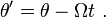
Linear acceleration. In the same manner, the acceleration of the object is defined as:
Two terminologies
In a purely mathematical treatment, regardless of the frame that the coordinate system is associated with (inertial or non-inertial), extra terms appear in the acceleration of an observed particle when using curvilinear coordinates. For example, in polar coordinates the acceleration is given by (see below for details):

Assuming it is clear that "state of motion" and "coordinate system" are different, it follows that the dependence of centrifugal force (as in this article) upon "state of motion" and its independence from "coordinate system", which contrasts with the "coordinate" version with exactly the opposite dependencies, indicates that two different ideas are referred to by the terminology "fictitious force". The present article emphasizes one of these two ideas ("state-of-motion"), although the other also is described.
Below, polar coordinates are introduced for use in (first) an inertial frame of reference and then (second) in a rotating frame of reference. The two different uses of the term "fictitious force" are pointed out. First, however, follows a brief digression to explain further how the "coordinate" terminology for fictitious force has arisen.
Lagrangian approach
To motivate the introduction of "coordinate" inertial forces by more than a reference to "mathematical convenience", what follows is a digression to show these forces correspond to what are called by some authors "generalized" fictitious forces or "generalized inertia forces". These forces are introduced via the Lagrangian mechanics approach to mechanics based upon describing a system by generalized coordinates usually denoted as {qk}. The only requirement on these coordinates is that they are necessary and sufficient to uniquely characterize the state of the system: they need not be (although they could be) the coordinates of the particles in the system. Instead, they could be the angles and extensions of links in a robot arm, for instance. If a mechanical system consists of N particles and there are m independent kinematical conditions imposed, it is possible to characterize the system uniquely by n = 3N - m independent generalized coordinates {qk}.
In classical mechanics, the Lagrangian is defined as the kinetic energy, T, of the system minus its potential energy, U. In symbols,

Here are some definitions:
- Definition:
- is the Lagrange function or Lagrangian, qi are the generalized coordinates,
 are generalized velocities,
 are generalized momenta,
 are generalized forces,
 are Lagrange's equations.

To proceed, consider a single particle, and introduce the generalized coordinates as {qk} = (r, θ). Then Hildebrand shows in polar coordinates with the qk = (r, θ) the "generalized momenta" are:

 Careful reading of Hildebrand shows he doesn't discuss the role of "inertial frames of reference", and in fact, says "[The] presence or absence [of inertia forces] depends, not upon the particular problem at hand but upon the coordinate system chosen." By coordinate system presumably is meant the choice of {qk}. Later he says "If accelerations associated with generalized coordinates are to be of prime interest (as is usually the case), the [nonaccelerational] terms may be conveniently transferred to the right … and considered as additional (generalized) inertia forces. Such inertia forces are often said to be of the Coriolis type."
In short, the emphasis of some authors upon coordinates and their derivatives and their introduction of (generalized) fictitious forces that do not vanish in inertial frames of reference is an outgrowth of the use of generalized coordinates in Lagrangian mechanics. For example, see McQuarrie. Hildebrand, and von Schwerin.Below is an example of this usage as employed in the design of robotic manipulators:
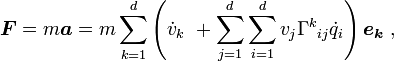
In the above [Lagrange-Euler] equations, there are three types of terms. The first involves the second derivative of the generalized co-ordinates. The second is quadratic inwhere the coefficients may depend on
. These are further classified into two types. Terms involving a product of the type
are called centrifugal forces while those involving a product of the type
for i ≠ j are called Coriolis forces. The third type is functions of
– Shuzhi S. Ge, Tong Heng Lee & Christopher John Harris: Adaptive Neural Network Control of Robotic Manipulators, pp. 47-48
For a robot manipulator, the equations may be written in a form using Christoffel symbols Γijk (discussed further below) as:
The introduction of generalized fictitious forces often is done without notification and without specifying the word "generalized". This sloppy use of terminology leads to endless confusion because these generalized fictitious forces, unlike the standard "state-of-motion" fictitious forces, do not vanish in inertial frames of reference.
Polar coordinates in an inertial frame of reference
Below, the acceleration of a particle is derived as seen in an inertial frame using polar coordinates. There are no "state-of-motion" fictitious forces in an inertial frame, by definition. Following that presentation, the contrasting terminology of "coordinate" fictitious forces is presented and critiqued on the basis of the non-vectorial transformation behavior of these "forces".
In an inertial frame, let
be the position vector of a moving particle. Its Cartesian components (x, y) are:
Unit vectors are defined in the radially outward direction
: :
:

 , in an inertial frame of reference Newton's second law expressed in polar coordinates is:
From a mathematical standpoint, however, it sometimes is handy to put only the second-order derivatives on the right side of this equation; that is we write the above equation by rearrangement of terms as:


These newly defined "forces" are non-zero in an inertial frame, and so certainly are not the same as the previously identified fictitious forces that are zero in an inertial frame and non-zero only in a non-inertial frame. In this article, these newly defined forces are called the "coordinate" centrifugal force and the "coordinate" Coriolis force to separate them from the "state-of-motion" forces.
Change of origin
 |
Figure 2: Two coordinate systems differing by a displacement of origin. Radial motion with constant velocity v in one frame is not radial in the other frame. Angular rate  , but , but  |
does not transform as a true force, putting any reference to this term not just as a "term", but as a centrifugal force, in a dubious light. Suppose in frame S a particle moves radially away from the origin at a constant velocity. See Figure 2. The force on the particle is zero by Newton's first law. Now we look at the same thing from frame S' , which is the same, but displaced in origin. In S' the particle still is in straight line motion at constant speed, so again the force is zero.What if we use polar coordinates in the two frames? In frame S the radial motion is constant and there is no angular motion. Hence, the acceleration is:
 and . There is no force, including no "force" in frame S. In frame S' , however, we have:
 nor is zero. That is, we cannot obtain zero force (zero ) if we retain only as the acceleration; we need both terms.
Despite the above facts, suppose we adopt polar coordinates, and wish to say that
is "centrifugal force", and reinterpret as "acceleration" (without dwelling upon any possible justification). How does this decision fare when we consider that a proper formulation of physics is geometry and coordinate-independent? See the article on general covariance. To attempt to form a covariant expression, this so-called centrifugal "force" can be put into vector notation as:
 a unit vector normal to the plane of motion. Unfortunately, although this expression formally looks like a vector, when an observer changes origin the value of changes (see Figure 2), so observers in the same frame of reference standing on different street corners see different "forces" even though the actual events they witness are identical. How can a physical force (be it fictitious or real) be zero in one frame S, but non-zero in another frame S' identical, but a few feet away? Even for exactly the same particle behavior the expression is different in every frame of reference, even for very trivial distinctions between frames. In short, if we take as "centrifugal force", it does not have a universal significance: it is unphysical.
Beyond this problem, the real impressed net force is zero. (There is no real impressed force in straight-line motion at constant speed). If we adopt polar coordinates, and wish to say that
is "centrifugal force", and reinterpret as "acceleration", the oddity results in frame S' that straight-line motion at constant speed requires a net force in polar coordinates, but not in Cartesian coordinates. Moreover, this perplexity applies in frame S', but not in frame S.The absurdity of the behavior of
indicates that one must say that is not centrifugal force, but simply one of two terms in the acceleration. This view, that the acceleration is composed of two terms, is frame-independent: there is zero centrifugal force in any and every inertial frame. It also is coordinate-system independent: we can use Cartesian, polar, or any other curvilinear system: they all produce zero.Apart from the above physical arguments, of course, the derivation above, based upon application of the mathematical rules of differentiation, shows the radial acceleration does indeed consist of the two terms
.That said, the next subsection shows there is a connection between these centrifugal and Coriolis terms and the fictitious forces that pertain to a particular rotating frame of reference (as distinct from an inertial frame).
Co-rotating frame
 |
| Figure 3: Inertial frame of reference S and instantaneous non-inertial co-rotating frame of reference S' . The co-rotating frame rotates at angular rate Ω equal to the rate of rotation of the particle about the origin of S' at the particular moment t. Particle is located at vector position r(t) and unit vectors are shown in the radial direction to the particle from the origin, and also in the direction of increasing angle θ normal to the radial direction. These unit vectors need not be related to the tangent and normal to the path. Also, the radial distance r need not be related to the radius of curvature of the path. |
Polar coordinates in a rotating frame of reference
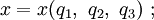
Next, the same approach is used to find the fictitious forces of a (non-inertial) rotating frame. For example, if a rotating polar coordinate system is adopted for use in a rotating frame of observation, both rotating at the same constant counterclockwise rate Ω, we find the equations of motion in this frame as follows: the radial coordinate in the rotating frame is taken as r, but the angle θ' in the rotating frame changes with time:


 is the radial component of the Coriolis force per unit mass, where is the tangential component of the particle velocity as seen in the rotating frame. The term is the so-called azimuthal component of the Coriolis force per unit mass. In fact, these extra terms can be used to measure Ω and provide a test to see whether or not the frame is rotating, just as explained in the example of rotating identical spheres. If the particle's motion can be described by the observer using Newton's laws of motion without these Ω-dependent terms, the observer is in an inertial frame of reference where Ω=0.
These "extra terms" in the acceleration of the particle are the "state of motion" fictitious forces for this rotating frame, the forces introduced by rotation of the frame at angular rate Ω.
In this rotating frame, what are the "coordinate" fictitious forces? As before, suppose we choose to put only the second-order time derivatives on the right side of Newton's law:


 as some so-called "acceleration", then the terms are added to the so-called "fictitious force", which are not "state-of-motion" fictitious forces, but are actually components of force that persist even when Ω=0, that is, they persist even in an inertial frame of reference. Because these extra terms are added, the "coordinate" fictitious force is not the same as the "state-of-motion" fictitious force. Because of these extra terms, the "coordinate" fictitious force is not zero even in an inertial frame of reference.
More on the co-rotating frame
Notice however, the case of a rotating frame that happens to have the same angular rate as the particle, so that Ω = dθ/dt at some particular moment (that is, the polar coordinates are set up in the instantaneous, non-inertial co-rotating frame of Figure 3). In this case, at this moment, dθ'/dt = 0. In this co-rotating non-inertial frame at this moment the "coordinate" fictitious forces are only those due to the motion of the frame, that is, they are the same as the "state-of-motion" fictitious forces, as discussed in the remarks about the co-rotating frame of Figure 3 in the previous section.
Fictitious forces in curvilinear coordinates
 |
| Figure 4: Coordinate surfaces, coordinate lines, and coordinate axes of general curvilinear coordinates |
Instead of Cartesian coordinates, when equations of motion are expressed in a curvilinear coordinate system, Christoffel symbols appear in the acceleration of a particle expressed in this coordinate system, as described below in more detail. Consider description of a particle motion from the viewpoint of an inertial frame of reference in curvilinear coordinates. Suppose the position of a point P in Cartesian coordinates is (x, y, z) and in curvilinear coordinates is (q1, q2. q3). Then functions exist that relate these descriptions:


 or, in general,


Using relations like this one,


"State-of-motion" versus "coordinate" fictitious forces
Earlier in this article a distinction was introduced between two terminologies, the fictitious forces that vanish in an inertial frame of reference are called in this article the "state-of-motion" fictitious forces and those that originate from differentiation in a particular coordinate system are called "coordinate" fictitious forces. Using the expression for the acceleration above, Newton's law of motion in the inertial frame of reference becomes:
The "coordinate" approach to Newton's law above is to retain the second-order time derivatives of the coordinates {qk} as the only terms on the right side of this equation, motivated more by mathematical convenience than by physics. To that end, the force law can be rewritten, taking the second summation to the force-side of the equation as:
 is now:
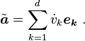
If the frame is not inertial, for example, in a rotating frame of reference, the "state-of-motion" fictitious forces are included in the above "coordinate" fictitious force expression. Also, if the "acceleration" expressed in terms of first-order time derivatives of the velocity happens to result in terms that are not simply second-order derivatives of the coordinates {qk} in time, then these terms that are not second-order also are brought to the force-side of the equation and included with the fictitious forces. From the standpoint of a Lagrangian formulation, they can be called generalized fictitious forces. See Hildebrand , for example.
Formulation of dynamics in terms of Christoffel symbols and the "coordinate" version of fictitious forces is used often in the design of robots in connection with a Lagrangian formulation of the equations of motion.
Particle Kinematics
Position & Reference Frames
The position of a point in space is the most fundamental idea in particle kinematics. To specify the position of a point, one must specify three things: the reference point (often called the origin), distance from the reference point and the direction in space of the straight line from the reference point to the particle. Exclusion of any of these three parameters renders the description of position incomplete. Consider for example a tower 50 m south from your home. The reference point is home, the distance 50 m and the direction south. If one only says that the tower is 50 m south, the natural question that arises is "from where?" If one says that the tower is southward from your home, the question that arises is "how far?" If one says the tower is 50 m from your home, the question that arises is "in which direction?" Hence, all these three parameters are crucial to defining uniquely the position of a point in space.
Position is usually described by mathematical quantities that have all these three attributes: the most common are vectors and complex numbers. Usually, only vectors are used. For measurement of distances and directions, usually three dimensional coordinate systems are used with the origin coinciding with the reference point. A three-dimensional coordinate system (whose origin coincides with the reference point) with some provision for time measurement is called a reference frame or frame of reference or simply frame. All observations in physics are incomplete without the reference frame being specified.
Position Vector
The position vector of a particle is a vector drawn from the origin of the reference frame to the particle. It expresses both the distance of the point from the origin and its sense from the origin. In three dimensions, the position of point A can be expressed as

Rest & Motion
Once the notion of position is firmly established, the ideas of rest and motion naturally follow. If the position vector of the particle (relative to a given reference frame) changes with time, then the particle is said to be in motion with respect to the chosen reference frame. However, if the position vector of the particle (relative to a given reference frame) remains the same with time, then the particle is said to be at rest with respect to the chosen frame. Note that rest and motion are relative to the reference frame chosen. It is quite possible that a particle at rest relative to a particular reference frame is in motion relative to the other. Hence, rest and motion aren't absolute terms, rather they are dependent on reference frame. For example, a passenger in a moving car may be at rest with respect to the car, but in motion with respect to the road.
Path
A particle's path is the locus between its beginning and end points which is reference-frame dependent. The path of a particle may be rectilinear (straight line) in one frame, and curved in another.
Displacement
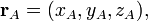
Displacement is a vector describing the difference in position between two points, i.e. it is the change in position the particle undergoes during the time interval. If point A has position rA = (xA,yA,zA) and point B has position rB = (xB,yB,zB), the displacement rAB of B from A is given by

Distance
 |
| The distance traveled is always greater than or equal to the displacement |
When considering the motion of a particle over time, distance is the length of the particle's path and may be different from displacement, which is the change from its initial position to its final position. For example, a race car traversing a 10 km closed loop from start to finish travels a distance of 10 km; its displacement, however, is zero because it arrives back at its initial position.
If the position of the particle is known as a function of time (r = r(t)), the distance s it travels from time t1 to time t2 can be found by

Velocity and speed
Average velocity is defined as

Velocity is the measure of the rate of change in position with respect to time, that is, how the distance of a point changes with each instant of time. Velocity also is a vector. Instantaneous velocity (the velocity at an instant of time) can be defined as the limiting value of average velocity as the time interval Δt becomes smaller and smaller. Both Δr and Δt approach zero but the ratio v approaches a non-zero limit v. That is,
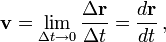
As a position vector itself is frame dependent, velocity is also dependent on the reference frame.
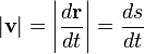
The speed of an object is the magnitude |v| of its velocity. It is a scalar quantity:
Acceleration
Average acceleration (acceleration over a length of time) is defined as:

Acceleration is the vector quantity describing the rate of change with time of velocity. Instantaneous acceleration (the acceleration at an instant of time) is defined as the limiting value of average acceleration as Δt becomes smaller and smaller. Under such a limit, a → a.

Types of motion based on velocity and acceleration
If the acceleration of a particle is zero, then the velocity of the particle is constant over time and the motion is said to be uniform. Otherwise, the motion is non-uniform.
If the acceleration is non-zero but constant, the motion is said to be motion with constant acceleration. On the other hand, if the acceleration is variable, the motion is called motion with variable acceleration. In motion with variable acceleration, the rate of change of acceleration is called the jerk.
Integral relations
The above definitions can be inverted by mathematical integration to find:

![\begin{align}
\mathbf{r}(t) &=\mathbf{r}_0 + \int_{t_0}^t \mathbf{v}(t) \; dt \\
&= \mathbf{r}_0 + \mathbf{v}_0 t + \int_{t_0}^t \left[\int_{t_0}^{t} \mathbf{a}(t) dt \right]\; dt \\
\end{align}](http://upload.wikimedia.org/math/0/1/0/01094ba0d9d835f5421ae08ed1964392.png)
Kinematics of constant acceleration
Many physical situations can be modeled as constant-acceleration processes, such as projectile motion.
Integrating acceleration a with respect to time t gives the change in velocity. When acceleration is constant both in direction and in magnitude, the point is said to be undergoing uniformly accelerated motion. In this case, the integral relations can be simplified:


A relationship without explicit time dependence may also be derived for one-dimensional motion. Noting that at = v − v0,


Relative velocity
To describe the motion of object A with respect to object B, when we know how each is moving with respect to a reference object O, we can use vector algebra. Choose an origin for reference, and let the positions of objects A, B, and O be denoted by rA, rB, and rO. Then the position of A relative to the reference object O is

For example, let Ann move with velocity
relative to the reference (we drop the O subscript for convenience) and let Bob move with velocity , each velocity given with respect to the ground (point O). To find how fast Ann is moving relative to Bob (we call this velocity ), the equation above gives: we simply rearrange this equation to obtain:
Example: Rectilinear (1D) motion
 |
| Figure A: An object is fired upwards, reaches its apex, and then begins its descent under a constant acceleration. Note: The equations described here holds for object fired from ground and should not be mistaken with this picture |
.
For the sake of example, assume the object has an initial velocity of +50 m s−1. There are several interesting kinematic questions we can ask about the particle's motion:
- How long will it be airborne?


- What altitude will it reach before it begins to fall?

- What will its final velocity be when it reaches the ground?

Example: Projectile (2D) motion
 | |
| Figure B: An object fired at an angle θ from the ground follows a parabolic trajectory. Note: The equations described here holds for object fired from ground and should not be mistaken with this picture |
- How far will it travel before hitting the ground?


Kinematics is the study of how things move. Here, we are interested in the motion of normal objects in our world. A normal object is visible, has edges, and has a location that can be expressed with (x, y, z) coordinates. We will not be discussing the motion of atomic particles or black holes or light.
We will create a vocabulary and a group of mathematical methods that will describe this ordinary motion. Understand that we will be developing a language for describing motion only. We won't be concerned with what is causing or changing the motion, or more correctly, the momentums of the objects. In other words, we are not concerned with the action of forces within this topic.
Rotational motion
 |
| Figure 1: The angular velocity vector Ω points up for counterclockwise rotation and down for clockwise rotation, as specified by the right-hand rule. Angular position θ(t) changes with time at a rate ω(t) = dθ/dt. |
Description of rotation then involves these three quantities:
- Angular position: The oriented distance from a selected origin on the rotational axis to a point of an object is a vector r ( t ) locating the point. The vector r(t) has some projection (or, equivalently, some component) r⊥(t) on a plane perpendicular to the axis of rotation. Then the angular position of that point is the angle θ from a reference axis (typically the positive x-axis) to the vector r⊥(t) in a known rotation sense (typically given by the right-hand rule).
- Angular velocity: The angular velocity ω is the rate at which the angular position θ changes with respect to time t:

- Angular acceleration: The magnitude of the angular acceleration α is the rate at which the angular velocity ω changes with respect to time t:


Point object in circular motion
 |
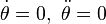
| Figure 2: Velocity and acceleration for nonuniform circular motion: the velocity vector is tangential to the orbit, but the acceleration vector is not radially inward because of its tangential component aθ that increases the rate of rotation: dω/dtaθ|/ = |R |
Displacement. An object in circular motion is located at a position r(t) given by:

Linear velocity. The velocity of the object is then


Linear acceleration. In the same manner, the acceleration of the object is defined as:
Coordinate systems
In any given situation, the most useful coordinates may be determined by constraints on the motion, or by the geometrical nature of the force causing or affecting the motion. Thus, to describe the motion of a bead constrained to move along a circular hoop, the most useful coordinate may be its angle on the hoop. Similarly, to describe the motion of a particle acted upon by a central force, the most useful coordinates may be polar coordinates. Polar coordinates are extended into three dimensions with either the spherical polar or cylindrical polar coordinate systems. These are most useful in systems exhibiting spherical or cylindrical symmetry respectively.
The position vector, r, the velocity vector, v, and the acceleration vector, a are expressed using rectangular coordinates in the following way:
 ,
, 
We know that:

 part. has two parts we want to find the derivative of: the relative change in velocity (
 ), and the change in the coordinate frame
( ).
).
 . Using the chain rule:
A kinematic constraint is any condition relating properties of a dynamic system that must hold true at all times. Below are some common examples:
Fixed rectangular coordinates
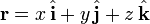
In this coordinate system, vectors are expressed as an addition of vectors in the x, y, and z direction from a non-rotating origin. Usually i, j, k are unit vectors in the x-, y-, and z-directions.
The position vector, r, the velocity vector, v, and the acceleration vector, a are expressed using rectangular coordinates in the following way:

 ,
, Two dimensional rotating reference frame
This coordinate system expresses only planar motion. It is based on three orthogonal unit vectors: the vector i, and the vector j which form a basis for the plane in which the objects we are considering reside, and k about which rotation occurs. Unlike rectangular coordinates, which are measured relative to an origin that is fixed and non-rotating, the origin of these coordinates can rotate and translate - often following a particle on a body that is being studied.
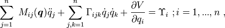
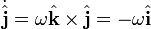
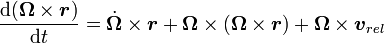
Derivatives of unit vectors
The position, velocity, and acceleration vectors of a given point can be expressed using these coordinate systems, but we have to be a bit more careful than we do with fixed frames of reference. Since the frame of reference is rotating, the unit vectors also rotate, and this rotation must be taken into account when taking the derivative of any of these vectors. If the coordinate frame is rotating at angular rate ω in the counterclockwise direction (that is, Ω = ω k using the right hand rule) then the derivatives of the unit vectors are as follows:

Position, velocity, and acceleration
Given these identities, we can now figure out how to represent the position, velocity, and acceleration vectors of a particle using this reference frame.
Position
Position is straightforward:
Velocity
Velocity is the time derivative of position: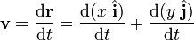


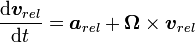
Acceleration
Acceleration is the time derivative of velocity.We know that:
 part. has two parts we want to find the derivative of: the relative change in velocity (), and the change in the coordinate frame
(
). . Using the chain rule:
 from above:


Kinematic constraints
Rolling without slipping
An object that rolls against a surface without slipping obeys the condition that the velocity of its center of mass is equal to the cross product of its angular velocity with a vector from the point of contact to the center of mass,
 .
.
Inextensible cord
This is the case where bodies are connected by an idealized cord that remains in tension and cannot change length. The constraint is that the sum of lengths of all segments of the cord is the total length, and accordingly the time derivative of this sum is zero. See Kelvin and Tait and Fogiel. A dynamic problem of this type is the pendulum. Another example is a drum turned by the pull of gravity upon a falling weight attached to the rim by the inextensible cord. An equilibrium problem (not kinematic) of this type is the catenary.
DYNAMICS (Mechanics)
In the field of physics, the study of the causes of motion and changes in motion is dynamics. In other words the study of forces and why objects are in motion. Dynamics includes the study of the effect of torques on motion. These are in contrast to Kinematics, the branch of classical mechanics that describes the motion of objects without consideration of the causes leading to the motion.
Generally speaking, researchers involved in dynamics study how a physical system might develop or alter over time and study the causes of those changes. In addition, Isaac Newton established the undergirding physical laws which govern dynamics in physics. By studying his system of mechanics, dynamics can be understood. In particular dynamics is mostly related to Newton's second law of motion. However, all three laws of motion are taken into consideration, because these are interrelated in any given observation or experiment.
For classical electromagnetism, it is Maxwell's equations that describe the dynamics. And the dynamics of classical systems involving both mechanics and electromagnetism are described by the combination of Newton's laws, Maxwell's equations, and the Lorentz force.
Force
In physics, a force is any influence that causes a free body to undergo a change in speed, a change in direction, or a change in shape. Force can also be described by intuitive concepts such as a push or pull that can cause an object with mass to change its velocity (which includes to begin moving from a state of rest), i.e., to accelerate, or which can cause a flexible object to deform. A force has both magnitude and direction, making it a vector quantity. Newton's second law, F=ma, can be formulated to state that an object with a constant mass will accelerate in proportion to the net force acting upon and in inverse proportion to its mass, an approximation which breaks down near the speed of light. Newton's original formulation is exact, and does not break down: this version states that the net force acting upon an object is equal to the rate at which its momentum changes.
Related concepts to accelerating forces include thrust, increasing the velocity of the object, drag, decreasing the velocity of any object, and torque, causing changes in rotational speed about an axis. Forces which do not act uniformly on all parts of a body will also cause mechanical stresses, a technical term for influences which cause deformation of matter. While mechanical stress can remain embedded in a solid object, gradually deforming it, mechanical stress in a fluid determines changes in its pressure and volume.
Philosophers in antiquity used the concept of force in the study of stationary and moving objects and simple machines, but thinkers such as Aristotle and Archimedes retained fundamental errors in understanding force. In part this was due to an incomplete understanding of the sometimes non-obvious force of friction, and a consequently inadequate view of the nature of natural motion. A fundamental error was the belief that a force is required to maintain motion, even at a constant velocity. Most of the previous misunderstandings about motion and force were eventually corrected by Sir Isaac Newton; with his mathematical insight, he formulated laws of motion that remained unchanged for nearly three hundred years. By the early 20th century, Einstein developed a theory of relativity that correctly predicted the action of forces on objects with increasing momenta near the speed of light, and also provided insight into the forces produced by gravitation and inertia.
With modern insights into quantum mechanics and technology that can accelerate particles close to the speed of light, particle physics has devised a Standard Model to describe forces between particles smaller than atoms. The Standard Model predicts that exchanged particles called gauge bosons are the fundamental means by which forces are emitted and absorbed. Only four main interactions are known: in order of decreasing strength, they are: strong, electromagnetic, weak, and gravitational. High-energy particle physics observations made during the 1970s and 1980s confirmed that the weak and electromagnetic forces are expressions of a more fundamental electroweak interaction
Forces act in a particular direction and have sizes dependent upon how strong the push or pull is. Because of these characteristics, forces are classified as "vector quantities". This means that forces follow a different set of mathematical rules than physical quantities that do not have direction (denoted scalar quantities). For example, when determining what happens when two forces act on the same object, it is necessary to know both the magnitude and the direction of both forces to calculate the result. If both of these pieces of information are not known for each force, the situation is ambiguous. For example, if you know that two people are pulling on the same rope with known magnitudes of force but you do not know which direction either person is pulling, it is impossible to determine what the acceleration of the rope will be. The two people could be pulling against each other as in tug of war or the two people could be pulling in the same direction. In this simple one-dimensional example, without knowing the direction of the forces it is impossible to decide whether the net force is the result of adding the two force magnitudes or subtracting one from the other. Associating forces with vectors avoids such problems.
Historically, forces were first quantitatively investigated in conditions of static equilibrium where several forces canceled each other out. Such experiments demonstrate the crucial properties that forces are additive vector quantities: they have magnitude and direction. When two forces act on an object, the resulting force, the resultant (also called the net force), can be determined by following the parallelogram rule of vector addition: the addition of two vectors represented by sides of a parallelogram, gives an equivalent resultant vector which is equal in magnitude and direction to the transversal of the parallelogram. The magnitude of the resultant varies from the difference of the magnitudes of the two forces to their sum, depending on the angle between their lines of action.
Free-body diagrams can be used as a convenient way to keep track of forces acting on a system. Ideally, these diagrams are drawn with the angles and relative magnitudes of the force vectors preserved so that graphical vector addition can be done to determine the resultant.
As well as being added, forces can also be resolved into independent components at right angles to each other. A horizontal force pointing northeast can therefore be split into two forces, one pointing north, and one pointing east. Summing these component forces using vector addition yields the original force. Resolving force vectors into components of a set of basis vectors is often a more mathematically clean way to describe forces than using magnitudes and directions. This is because, for orthogonal components, the components of the vector sum are uniquely determined by the scalar addition of the components of the individual vectors. Orthogonal components are independent of each other because forces acting at ninety degrees to each other have no effect on the magnitude or direction of the other. Choosing a set of orthogonal basis vectors is often done by considering what set of basis vectors will make the mathematics most convenient. Choosing a basis vector that is in the same direction as one of the forces is desirable, since that force would then have only one non-zero component. Orthogonal force vectors can be three-dimensional with the third component being at right-angles to the other two.
There are two kinds of equilibrium: static equilibrium and dynamic equilibrium.
The simplest case of static equilibrium occurs when two forces are equal in magnitude but opposite in direction. For example, an object on a level surface is pulled (attracted) downward toward the center of the Earth by the force of gravity. At the same time, surface forces resist the downward force with equal upward force (called the normal force). The situation is one of zero net force and no acceleration.
Pushing against an object on a frictional surface can result in a situation where the object does not move because the applied force is opposed by static friction, generated between the object and the table surface. For a situation with no movement, the static friction force exactly balances the applied force resulting in no acceleration. The static friction increases or decreases in response to the applied force up to an upper limit determined by the characteristics of the contact between the surface and the object.
A static equilibrium between two forces is the most usual way of measuring forces, using simple devices such as weighing scales and spring balances. For example, an object suspended on a vertical spring scale experiences the force of gravity acting on the object balanced by a force applied by the "spring reaction force" which equals object's weight. Using such tools, some quantitative force laws were discovered: that the force of gravity is proportional to volume for objects of constant density (widely exploited for millennia to define standard weights); Archimedes' principle for buoyancy; Archimedes' analysis of the lever; Boyle's law for gas pressure; and Hooke's law for springs. These were all formulated and experimentally verified before Isaac Newton expounded his three laws of motion.
Related concepts to accelerating forces include thrust, increasing the velocity of the object, drag, decreasing the velocity of any object, and torque, causing changes in rotational speed about an axis. Forces which do not act uniformly on all parts of a body will also cause mechanical stresses, a technical term for influences which cause deformation of matter. While mechanical stress can remain embedded in a solid object, gradually deforming it, mechanical stress in a fluid determines changes in its pressure and volume.
Philosophers in antiquity used the concept of force in the study of stationary and moving objects and simple machines, but thinkers such as Aristotle and Archimedes retained fundamental errors in understanding force. In part this was due to an incomplete understanding of the sometimes non-obvious force of friction, and a consequently inadequate view of the nature of natural motion. A fundamental error was the belief that a force is required to maintain motion, even at a constant velocity. Most of the previous misunderstandings about motion and force were eventually corrected by Sir Isaac Newton; with his mathematical insight, he formulated laws of motion that remained unchanged for nearly three hundred years. By the early 20th century, Einstein developed a theory of relativity that correctly predicted the action of forces on objects with increasing momenta near the speed of light, and also provided insight into the forces produced by gravitation and inertia.
With modern insights into quantum mechanics and technology that can accelerate particles close to the speed of light, particle physics has devised a Standard Model to describe forces between particles smaller than atoms. The Standard Model predicts that exchanged particles called gauge bosons are the fundamental means by which forces are emitted and absorbed. Only four main interactions are known: in order of decreasing strength, they are: strong, electromagnetic, weak, and gravitational. High-energy particle physics observations made during the 1970s and 1980s confirmed that the weak and electromagnetic forces are expressions of a more fundamental electroweak interaction
 |
| Forces are also described as a push or pull on an object. They can be due to phenomena such as gravity, magnetism, or anything that might cause a mass to accelerate |
Descriptions
Since forces are perceived as pushes or pulls, this can provide an intuitive understanding for describing forces. As with other physical concepts (e.g. temperature), the intuitive understanding of forces is quantified using precise operational definitions that are consistent with direct observations and compared to a standard measurement scale. Through experimentation, it is determined that laboratory measurements of forces are fully consistent with the conceptual definition of force offered by Newtonian mechanics.Forces act in a particular direction and have sizes dependent upon how strong the push or pull is. Because of these characteristics, forces are classified as "vector quantities". This means that forces follow a different set of mathematical rules than physical quantities that do not have direction (denoted scalar quantities). For example, when determining what happens when two forces act on the same object, it is necessary to know both the magnitude and the direction of both forces to calculate the result. If both of these pieces of information are not known for each force, the situation is ambiguous. For example, if you know that two people are pulling on the same rope with known magnitudes of force but you do not know which direction either person is pulling, it is impossible to determine what the acceleration of the rope will be. The two people could be pulling against each other as in tug of war or the two people could be pulling in the same direction. In this simple one-dimensional example, without knowing the direction of the forces it is impossible to decide whether the net force is the result of adding the two force magnitudes or subtracting one from the other. Associating forces with vectors avoids such problems.
Historically, forces were first quantitatively investigated in conditions of static equilibrium where several forces canceled each other out. Such experiments demonstrate the crucial properties that forces are additive vector quantities: they have magnitude and direction. When two forces act on an object, the resulting force, the resultant (also called the net force), can be determined by following the parallelogram rule of vector addition: the addition of two vectors represented by sides of a parallelogram, gives an equivalent resultant vector which is equal in magnitude and direction to the transversal of the parallelogram. The magnitude of the resultant varies from the difference of the magnitudes of the two forces to their sum, depending on the angle between their lines of action.
Free-body diagrams can be used as a convenient way to keep track of forces acting on a system. Ideally, these diagrams are drawn with the angles and relative magnitudes of the force vectors preserved so that graphical vector addition can be done to determine the resultant.
As well as being added, forces can also be resolved into independent components at right angles to each other. A horizontal force pointing northeast can therefore be split into two forces, one pointing north, and one pointing east. Summing these component forces using vector addition yields the original force. Resolving force vectors into components of a set of basis vectors is often a more mathematically clean way to describe forces than using magnitudes and directions. This is because, for orthogonal components, the components of the vector sum are uniquely determined by the scalar addition of the components of the individual vectors. Orthogonal components are independent of each other because forces acting at ninety degrees to each other have no effect on the magnitude or direction of the other. Choosing a set of orthogonal basis vectors is often done by considering what set of basis vectors will make the mathematics most convenient. Choosing a basis vector that is in the same direction as one of the forces is desirable, since that force would then have only one non-zero component. Orthogonal force vectors can be three-dimensional with the third component being at right-angles to the other two.
Equilibria
Equilibrium occurs when the resultant force acting on a point particle is zero (that is, the vector sum of all forces is zero). When dealing with an extended body, it is also necessary that the net torque in it is 0.
There are two kinds of equilibrium: static equilibrium and dynamic equilibrium.
Static equilibrium
Static equilibrium was understood well before the invention of classical mechanics. Objects which are at rest have zero net force acting on them.
The simplest case of static equilibrium occurs when two forces are equal in magnitude but opposite in direction. For example, an object on a level surface is pulled (attracted) downward toward the center of the Earth by the force of gravity. At the same time, surface forces resist the downward force with equal upward force (called the normal force). The situation is one of zero net force and no acceleration.
Pushing against an object on a frictional surface can result in a situation where the object does not move because the applied force is opposed by static friction, generated between the object and the table surface. For a situation with no movement, the static friction force exactly balances the applied force resulting in no acceleration. The static friction increases or decreases in response to the applied force up to an upper limit determined by the characteristics of the contact between the surface and the object.
A static equilibrium between two forces is the most usual way of measuring forces, using simple devices such as weighing scales and spring balances. For example, an object suspended on a vertical spring scale experiences the force of gravity acting on the object balanced by a force applied by the "spring reaction force" which equals object's weight. Using such tools, some quantitative force laws were discovered: that the force of gravity is proportional to volume for objects of constant density (widely exploited for millennia to define standard weights); Archimedes' principle for buoyancy; Archimedes' analysis of the lever; Boyle's law for gas pressure; and Hooke's law for springs. These were all formulated and experimentally verified before Isaac Newton expounded his three laws of motion.
Dynamical equilibrium
Dynamical equilibrium was first described by Galileo who noticed that certain assumptions of Aristotelian physics were contradicted by observations and logic. Galileo realized that simple velocity addition demands that the concept of an "absolute rest frame" did not exist. Galileo concluded that motion in a constant velocity was completely equivalent to rest. This was contrary to Aristotle's notion of a "natural state" of rest that objects with mass naturally approached. Simple experiments showed that Galileo's understanding of the equivalence of constant velocity and rest to be correct. For example, if a mariner dropped a cannonball from the crow's nest of a ship moving at a constant velocity, Aristotelian physics would have the cannonball fall straight down while the ship moved beneath it. Thus, in an Aristotelian universe, the falling cannonball would land behind the foot of the mast of a moving ship. However, when this experiment is actually conducted, the cannonball always falls at the foot of the mast, as if the cannonball knows to travel with the ship despite being separated from it. Since there is no forward horizontal force being applied on the cannonball as it falls, the only conclusion left is that the cannonball continues to move with the same velocity as the boat as it falls. Thus, no force is required to keep the cannonball moving at the constant forward velocity.
Moreover, any object traveling at a constant velocity must be subject to zero net force (resultant force). This is the definition of dynamical equilibrium: when all the forces on an object balance but it still moves at a constant velocity.
A simple case of dynamical equilibrium occurs in constant velocity motion across a surface with kinetic friction. In such a situation, a force is applied in the direction of motion while the kinetic friction force exactly opposes the applied force. This results in a net zero force, but since the object started with a non-zero velocity, it continues to move with a non-zero velocity. Aristotle misinterpreted this motion as being caused by the applied force. However, when kinetic friction is taken into consideration it is clear that there is no net force causing constant velocity motion.
Special relativity
In the special theory of relativity mass and energy are equivalent (as can be seen by calculating the work required to accelerate an object). When an object's velocity increases so does its energy and hence its mass equivalent (inertia). It thus requires more force to accelerate it the same amount than it did at a lower velocity. Newton's second law


- v is the velocity and
- c is the speed of light.
 moving in the
  direction is:
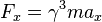


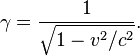
Relativistic force does not produce a constant acceleration, but an ever decreasing acceleration as the object approaches the speed of light. Note that γ is undefined for an object with a non zero rest mass at the speed of light, and the theory yields no prediction at that speed.
One can however restore the form of

Feynman diagrams
 |
| A Feynman diagram for the decay of a neutron into a proton. The W boson is between two vertices indicating a repulsion |
The utility of Feynman diagrams is that other types of physical phenomena that are part of the general picture of fundamental interactions but are conceptually separate from forces can also be described using the same rules. For example, a Feynman diagram can describe in succinct detail how a neutron decays into an electron, proton, and neutrino, an interaction mediated by the same gauge boson that is responsible for the weak nuclear force
Fundamental models
All the forces in the universe are based on four fundamental interactions. The strong and weak forces act only at very short distances, and are responsible for the interactions between subatomic particles including nucleons and compound nuclei. The electromagnetic force acts between electric charges and the gravitational force acts between masses. All other forces are based on the existence of the four fundamental interactions. For example, friction is a manifestation of the electromagnetic force acting between the atoms of two surfaces, and the Pauli Exclusion Principle, which does not allow atoms to pass through each other. The forces in springs, modeled by Hooke's law, are also the result of electromagnetic forces and the Exclusion Principle acting together to return the object to its equilibrium position. Centrifugal forces are acceleration forces which arise simply from the acceleration of rotating frames of reference.
The development of fundamental theories for forces proceeded along the lines of unification of disparate ideas. For example, Isaac Newton unified the force responsible for objects falling at the surface of the Earth with the force responsible for the orbits of celestial mechanics in his universal theory of gravitation. Michael Faraday and James Clerk Maxwell demonstrated that electric and magnetic forces were unified through one consistent theory of electromagnetism. In the twentieth century, the development of quantum mechanics led to a modern understanding that the first three fundamental forces (all except gravity) are manifestations of matter (fermions) interacting by exchanging virtual particles called gauge bosons. This standard model of particle physics posits a similarity between the forces and led scientists to predict the unification of the weak and electromagnetic forces in electroweak theory subsequently confirmed by observation. The complete formulation of the standard model predicts an as yet unobserved Higgs mechanism, but observations such as neutrino oscillations indicate that the standard model is incomplete. A grand unified theory allowing for the combination of the electroweak interaction with the strong force is held out as a possibility with candidate theories such as supersymmetry proposed to accommodate some of the outstanding unsolved problems in physics. Physicists are still attempting to develop self-consistent unification models that would combine all four fundamental interactions into a theory of everything. Einstein tried and failed at this endeavor, but currently the most popular approach to answering this question is string theory.
What we now call gravity was not identified as a universal force until the work of Isaac Newton. Before Newton, the tendency for objects to fall towards the Earth was not understood to be related to the motions of celestial objects. Galileo was instrumental in describing the characteristics of falling objects by determining that the acceleration of every object in free-fall was constant and independent of the mass of the object. Today, this acceleration due to gravity towards the surface of the Earth is usually designated as  and has a magnitude of about 9.81 meters per second squared (this measurement is taken from sea level and may vary depending on location), and points toward the center of the Earth. This observation means that the force of gravity on an object at the Earth's surface is directly proportional to the object's mass. Thus an object that has a mass of m will experience a force:
Newton's contribution to gravitational theory was to unify the motions of heavenly bodies, which Aristotle had assumed were in a natural state of constant motion, with falling motion observed on the Earth. He proposed a law of gravity that could account for the celestial motions that had been described earlier using Kepler's Laws of Planetary Motion.
Newton came to realize that the effects of gravity might be observed in different ways at larger distances. In particular, Newton determined that the acceleration of the Moon around the Earth could be ascribed to the same force of gravity if the acceleration due to gravity decreased as an inverse square law. Further, Newton realized that the acceleration due to gravity is proportional to the mass of the attracting body. Combining these ideas gives a formula that relates the mass ( ) and the radius (
 ) of the Earth to the gravitational acceleration:
 , the unit vector directed outward from the center of the Earth.
In this equation, a dimensional constant G is used to describe the relative strength of gravity. This constant has come to be known as Newton's Universal Gravitation Constant, though its value was unknown in Newton's lifetime. Not until 1798 was Henry Cavendish able to make the first measurement of G using a torsion balance; this was widely reported in the press as a measurement of the mass of the Earth since knowing the G could allow one to solve for the Earth's mass given the above equation. Newton, however, realized that since all celestial bodies followed the same laws of motion, his law of gravity had to be universal. Succinctly stated, Newton's Law of Gravitation states that the force on a spherical object of mass m1 due to the gravitational pull of mass m2 is
is the unit vector pointed in the direction away from the center of the first object toward the center of the second object.
This formula was powerful enough to stand as the basis for all subsequent descriptions of motion within the solar system until the twentieth century. During that time, sophisticated methods of perturbation analysis were invented to calculate the deviations of orbits due to the influence of multiple bodies on a planet, moon, comet, or asteroid. The formalism was exact enough to allow mathematicians to predict the existence of the planet Neptune before it was observed.
It was only the orbit of the planet Mercury that Newton's Law of Gravitation seemed not to fully explain. Some astrophysicists predicted the existence of another planet (Vulcan) that would explain the discrepancies; however, despite some early indications, no such planet could be found. When Albert Einstein finally formulated his theory of general relativity (GR) he turned his attention to the problem of Mercury's orbit and found that his theory added a correction which could account for the discrepancy. This was the first time that Newton's Theory of Gravity had been shown to be less correct than an alternative.
Since then, and so far, general relativity has been acknowledged as the theory which best explains gravity. In GR, gravitation is not viewed as a force, but rather, objects moving freely in gravitational fields travel under their own inertia in straight lines through curved space-time – defined as the shortest space-time path between two space-time events. From the perspective of the object, all motion occurs as if there were no gravitation whatsoever. It is only when observing the motion in a global sense that the curvature of space-time can be observed and the force is inferred from the object's curved path. Thus, the straight line path in space-time is seen as a curved line in space, and it is called the ballistic trajectory of the object. For example, a basketball thrown from the ground moves in a parabola, as it is in a uniform gravitational field. Its space-time trajectory (when the extra ct dimension is added) is almost a straight line, slightly curved (with the radius of curvature of the order of few light-years). The time derivative of the changing momentum of the object is what we label as "gravitational force".
Subsequent mathematicians and physicists found the construct of the electric field to be useful for determining the electrostatic force on an electric charge at any point in space. The electric field was based on using a hypothetical "test charge" anywhere in space and then using Coulomb's Law to determine the electrostatic force. Thus the electric field anywhere in space is defined as
Meanwhile, the Lorentz force of magnetism was discovered to exist between two electric currents. It has the same mathematical character as Coulomb's Law with the proviso that like currents attract and unlike currents repel. Similar to the electric field, the magnetic field can be used to determine the magnetic force on an electric current at any point in space. In this case, the magnitude of the magnetic field was determined to be
 is the length of hypothetical wire through which the test current flows. The magnetic field exerts a force on all magnets including, for example, those used in compasses. The fact that the Earth's magnetic field is aligned closely with the orientation of the Earth's axis causes compass magnets to become oriented because of the magnetic force pulling on the needle.
Through combining the definition of electric current as the time rate of change of electric charge, a rule of vector multiplication called Lorentz's Law describes the force on a charge moving in an magnetic field. The connection between electricity and magnetism allows for the description of a unified electromagnetic force that acts on a charge. This force can be written as a sum of the electrostatic force (due to the electric field) and the magnetic force (due to the magnetic field). Fully stated, this is the law:
 is the electromagnetic force, q is the magnitude of the charge of the particle,
  is the electric field,
  is the velocity of the particle which is crossed with the magnetic field (
 ).
).
The origin of electric and magnetic fields would not be fully explained until 1864 when James Clerk Maxwell unified a number of earlier theories into a set of 20 scalar equations, which were later reformulated into 4 vector equations by Oliver Heaviside and Willard Gibbs. These "Maxwell Equations" fully described the sources of the fields as being stationary and moving charges, and the interactions of the fields themselves. This led Maxwell to discover that electric and magnetic fields could be "self-generating" through a wave that traveled at a speed which he calculated to be the speed of light. This insight united the nascent fields of electromagnetic theory with optics and led directly to a complete description of the electromagnetic spectrum.
However, attempting to reconcile electromagnetic theory with two observations, the photoelectric effect, and the nonexistence of the ultraviolet catastrophe, proved troublesome. Through the work of leading theoretical physicists, a new theory of electromagnetism was developed using quantum mechanics. This final modification to electromagnetic theory ultimately led to quantum electrodynamics (or QED), which fully describes all electromagnetic phenomena as being mediated by wave particles known as photons. In QED, photons are the fundamental exchange particle which described all interactions relating to electromagnetism including the electromagnetic force.
It is a common misconception to ascribe the stiffness and rigidity of solid matter to the repulsion of like charges under the influence of the electromagnetic force. However, these characteristics actually result from the Pauli Exclusion Principle. Since electrons are fermions, they cannot occupy the same quantum mechanical state as other electrons. When the electrons in a material are densely packed together, there are not enough lower energy quantum mechanical states for them all, so some of them must be in higher energy states. This means that it takes energy to pack them together. While this effect is manifested macroscopically as a structural force, it is technically only the result of the existence of a finite set of electron states.
The strong force is today understood to represent the interactions between quarks and gluons as detailed by the theory of quantum chromodynamics (QCD). The strong force is the fundamental force mediated by gluons, acting upon quarks, antiquarks, and the gluons themselves. The (aptly named) strong interaction is the "strongest" of the four fundamental forces.
The strong force only acts directly upon elementary particles. However, a residual of the force is observed between hadrons (the best known example being the force that acts between nucleons in atomic nuclei) as the nuclear force. Here the strong force acts indirectly, transmitted as gluons which form part of the virtual pi and rho mesons which classically transmit the nuclear force (see this topic for more). The failure of many searches for free quarks has shown that the elementary particles affected are not directly observable. This phenomenon is called colour confinement.
The weak force is due to the exchange of the heavy W and Z bosons. Its most familiar effect is beta decay (of neutrons in atomic nuclei) and the associated radioactivity. The word "weak" derives from the fact that the field strength is some 1013 times less than that of the strong force. Still, it is stronger than gravity over short distances. A consistent electroweak theory has also been developed which shows that electromagnetic forces and the weak force are indistinguishable at a temperatures in excess of approximately 1015 kelvins. Such temperatures have been probed in modern particle accelerators and show the conditions of the universe in the early moments of the Big Bang.
The normal force is the repulsive force of interaction between atoms at close contact. When their electron clouds overlap, Pauli repulsion (due to fermionic nature of electrons) follows resulting in the force which acts normal to the surface interface between two objects. The normal force, for example, is responsible for the structural integrity of tables and floors as well as being the force that responds whenever an external force pushes on a solid object. An example of the normal force in action is the impact force on an object crashing into an immobile surface.
The static friction force (Fsf) will exactly oppose forces applied to an object parallel to a surface contact up to the limit specified by the coefficient of static friction (μsf) multiplied by the normal force (FN). In other words the magnitude of the static friction force satisfies the inequality:
An elastic force acts to return a spring to its natural length. An ideal spring is taken to be massless, frictionless, unbreakable, and infinitely stretchable. Such springs exert forces that push when contracted, or pull when extended, in proportion to the displacement of the spring from its equilibrium position. This linear relationship was described by Robert Hooke in 1676, for whom Hooke's law is named. If Δx is the displacement, the force exerted by an ideal spring equals:
Newton's laws and Newtonian mechanics in general were first developed to describe how forces affect idealized point particles rather than three-dimensional objects. However, in real life, matter has extended structure and forces that act on one part of an object might affect other parts of an object. For situations where lattice holding together the atoms in an object is able to flow, contract, expand, or otherwise change shape, the theories of continuum mechanics describe the way forces affect the material. For example, in extended fluids, differences in pressure result in forces being directed along the pressure gradients as follows:
A specific instance of such a force that is associated with dynamic pressure is fluid resistance: a body force that resists the motion of an object through a fluid due to viscosity. For so-called "Stokes' drag" the force is approximately proportional to the velocity, but opposite in direction:
In general relativity, gravity becomes a fictitious force that arises in situations where spacetime deviates from a flat geometry. As an extension, Kaluza-Klein theory and string theory ascribe electromagnetism and the other fundamental forces respectively to the curvature of differently scaled dimensions, which would ultimately imply that all forces are fictitious.
Forces that cause extended objects to rotate are associated with torques. Mathematically, the torque on a particle is defined as the cross-product:
Equivalently, the differential form of Newton's Second Law provides an alternative definition of torque:
 is the angular momentum of the particle.
Newton's Third Law of Motion requires that all objects exerting torques themselves experience equal and opposite torques, and therefore also directly implies the conservation of angular momentum for closed systems that experience rotations and revolutions through the action of internal torques.
is the unit vector pointing in the radial direction outwards from the center. This means that the unbalanced centripetal force felt by any object is always directed toward the center of the curving path. Such forces act perpendicular to the velocity vector associated with the motion of an object, and therefore do not change the speed of the object (magnitude of the velocity), but only the direction of the velocity vector. The unbalanced force that accelerates an object can be resolved into a component that is perpendicular to the path, and one that is tangential to the path. This yields both the tangential force which accelerates the object by either slowing it down or speeding it up and the radial (centripetal) force which changes its direction.
Similarly, integrating with respect to position gives a definition for the work done by a force:
Power P is the rate of change dW/dt of the work W, as the trajectory is extended by a position change in a time interval dt:
 the velocity.
Potential energy
Instead of a force, often the mathematically related concept of a potential energy field can be used for convenience. For instance, the gravitational force acting upon an object can be seen as the action of the gravitational field that is present at the object's location. Restating mathematically the definition of energy (via the definition of work), a potential scalar field is defined as that field whose gradient is equal and opposite to the force produced at every point:
Conservative forces include gravity, the electromagnetic force, and the spring force. Each of these forces has models which are dependent on a position often given as a radial vector emanating from spherically symmetric potentials. Examples of this follow:
For gravity:
For electrostatic forces:
For spring forces:
The connection between macroscopic non-conservative forces and microscopic conservative forces is described by detailed treatment with statistical mechanics. In macroscopic closed systems, nonconservative forces act to change the internal energies of the system, and are often associated with the transfer of heat. According to the Second Law of Thermodynamics, nonconservative forces necessarily result in energy transformations within closed systems from ordered to more random conditions as entropy increases.
The gravitational foot-pound-second English unit of force is the pound-force (lbf), defined as the force exerted by gravity on a pound-mass in the standard gravitational field of 9.80665 m·s−2. The pound-force provides an alternative unit of mass: one slug is the mass that will accelerate by one foot per second squared when acted on by one pound-force.
An alternative unit of force in a different foot-pound-second system, the absolute fps system, is the poundal, defined as the force required to accelerate a one pound mass at a rate of one foot per second squared. The units of slug and poundal are designed to avoid a constant of proportionality in Newton's second law.
The pound-force has a metric counterpart, less commonly used than the newton: the kilogram-force (kgf) (sometimes kilopond), is the force exerted by standard gravity on one kilogram of mass. The kilogram-force leads to an alternate, but rarely used unit of mass: the metric slug (sometimes mug or hyl) is that mass which accelerates at 1 m·s−2 when subjected to a force of 1 kgf. The kilogram-force is not a part of the modern SI system, and is generally deprecated; however it still sees use for some purposes as expressing jet thrust, bicycle spoke tension, torque wrench settings and engine output torque. Other arcane units of force include the sthène which is equivalent to 1000 N and the kip which is equivalent to 1000 lbf.
The development of fundamental theories for forces proceeded along the lines of unification of disparate ideas. For example, Isaac Newton unified the force responsible for objects falling at the surface of the Earth with the force responsible for the orbits of celestial mechanics in his universal theory of gravitation. Michael Faraday and James Clerk Maxwell demonstrated that electric and magnetic forces were unified through one consistent theory of electromagnetism. In the twentieth century, the development of quantum mechanics led to a modern understanding that the first three fundamental forces (all except gravity) are manifestations of matter (fermions) interacting by exchanging virtual particles called gauge bosons. This standard model of particle physics posits a similarity between the forces and led scientists to predict the unification of the weak and electromagnetic forces in electroweak theory subsequently confirmed by observation. The complete formulation of the standard model predicts an as yet unobserved Higgs mechanism, but observations such as neutrino oscillations indicate that the standard model is incomplete. A grand unified theory allowing for the combination of the electroweak interaction with the strong force is held out as a possibility with candidate theories such as supersymmetry proposed to accommodate some of the outstanding unsolved problems in physics. Physicists are still attempting to develop self-consistent unification models that would combine all four fundamental interactions into a theory of everything. Einstein tried and failed at this endeavor, but currently the most popular approach to answering this question is string theory.
Gravity
 |
| An initially stationary object which is allowed to fall freely under gravity drops a distance which is proportional to the square of the elapsed time. An image was taken 20 flashes per second. During the first 1/20th of a second the ball drops one unit of distance (here, a unit is about 12 mm); by 2/20ths it has dropped a total of 4 units; by 3/20ths, 9 units and so on |
.
and has a magnitude of about 9.81 meters per second squared (this measurement is taken from sea level and may vary depending on location), and points toward the center of the Earth. This observation means that the force of gravity on an object at the Earth's surface is directly proportional to the object's mass. Thus an object that has a mass of m will experience a force:
Newton's contribution to gravitational theory was to unify the motions of heavenly bodies, which Aristotle had assumed were in a natural state of constant motion, with falling motion observed on the Earth. He proposed a law of gravity that could account for the celestial motions that had been described earlier using Kepler's Laws of Planetary Motion.
Newton came to realize that the effects of gravity might be observed in different ways at larger distances. In particular, Newton determined that the acceleration of the Moon around the Earth could be ascribed to the same force of gravity if the acceleration due to gravity decreased as an inverse square law. Further, Newton realized that the acceleration due to gravity is proportional to the mass of the attracting body. Combining these ideas gives a formula that relates the mass (
) and the radius () of the Earth to the gravitational acceleration: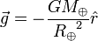 , the unit vector directed outward from the center of the Earth.
In this equation, a dimensional constant G is used to describe the relative strength of gravity. This constant has come to be known as Newton's Universal Gravitation Constant, though its value was unknown in Newton's lifetime. Not until 1798 was Henry Cavendish able to make the first measurement of G using a torsion balance; this was widely reported in the press as a measurement of the mass of the Earth since knowing the G could allow one to solve for the Earth's mass given the above equation. Newton, however, realized that since all celestial bodies followed the same laws of motion, his law of gravity had to be universal. Succinctly stated, Newton's Law of Gravitation states that the force on a spherical object of mass m1 due to the gravitational pull of mass m2 is
 is the unit vector pointed in the direction away from the center of the first object toward the center of the second object.
This formula was powerful enough to stand as the basis for all subsequent descriptions of motion within the solar system until the twentieth century. During that time, sophisticated methods of perturbation analysis were invented to calculate the deviations of orbits due to the influence of multiple bodies on a planet, moon, comet, or asteroid. The formalism was exact enough to allow mathematicians to predict the existence of the planet Neptune before it was observed.
It was only the orbit of the planet Mercury that Newton's Law of Gravitation seemed not to fully explain. Some astrophysicists predicted the existence of another planet (Vulcan) that would explain the discrepancies; however, despite some early indications, no such planet could be found. When Albert Einstein finally formulated his theory of general relativity (GR) he turned his attention to the problem of Mercury's orbit and found that his theory added a correction which could account for the discrepancy. This was the first time that Newton's Theory of Gravity had been shown to be less correct than an alternative.
Since then, and so far, general relativity has been acknowledged as the theory which best explains gravity. In GR, gravitation is not viewed as a force, but rather, objects moving freely in gravitational fields travel under their own inertia in straight lines through curved space-time – defined as the shortest space-time path between two space-time events. From the perspective of the object, all motion occurs as if there were no gravitation whatsoever. It is only when observing the motion in a global sense that the curvature of space-time can be observed and the force is inferred from the object's curved path. Thus, the straight line path in space-time is seen as a curved line in space, and it is called the ballistic trajectory of the object. For example, a basketball thrown from the ground moves in a parabola, as it is in a uniform gravitational field. Its space-time trajectory (when the extra ct dimension is added) is almost a straight line, slightly curved (with the radius of curvature of the order of few light-years). The time derivative of the changing momentum of the object is what we label as "gravitational force".
Electromagnetic forces
The electrostatic force was first described in 1784 by Coulomb as a force which existed intrinsically between two charges. The properties of the electrostatic force were that it varied as an inverse square law directed in the radial direction, was both attractive and repulsive (there was intrinsic polarity), was independent of the mass of the charged objects, and followed the superposition principle. Coulomb's Law unifies all these observations into one succinct statement.
Subsequent mathematicians and physicists found the construct of the electric field to be useful for determining the electrostatic force on an electric charge at any point in space. The electric field was based on using a hypothetical "test charge" anywhere in space and then using Coulomb's Law to determine the electrostatic force. Thus the electric field anywhere in space is defined as

Meanwhile, the Lorentz force of magnetism was discovered to exist between two electric currents. It has the same mathematical character as Coulomb's Law with the proviso that like currents attract and unlike currents repel. Similar to the electric field, the magnetic field can be used to determine the magnetic force on an electric current at any point in space. In this case, the magnitude of the magnetic field was determined to be
 is the length of hypothetical wire through which the test current flows. The magnetic field exerts a force on all magnets including, for example, those used in compasses. The fact that the Earth's magnetic field is aligned closely with the orientation of the Earth's axis causes compass magnets to become oriented because of the magnetic force pulling on the needle.
Through combining the definition of electric current as the time rate of change of electric charge, a rule of vector multiplication called Lorentz's Law describes the force on a charge moving in an magnetic field. The connection between electricity and magnetism allows for the description of a unified electromagnetic force that acts on a charge. This force can be written as a sum of the electrostatic force (due to the electric field) and the magnetic force (due to the magnetic field). Fully stated, this is the law:
 is the electromagnetic force, q is the magnitude of the charge of the particle, is the electric field, is the velocity of the particle which is crossed with the magnetic field ().
The origin of electric and magnetic fields would not be fully explained until 1864 when James Clerk Maxwell unified a number of earlier theories into a set of 20 scalar equations, which were later reformulated into 4 vector equations by Oliver Heaviside and Willard Gibbs. These "Maxwell Equations" fully described the sources of the fields as being stationary and moving charges, and the interactions of the fields themselves. This led Maxwell to discover that electric and magnetic fields could be "self-generating" through a wave that traveled at a speed which he calculated to be the speed of light. This insight united the nascent fields of electromagnetic theory with optics and led directly to a complete description of the electromagnetic spectrum.
However, attempting to reconcile electromagnetic theory with two observations, the photoelectric effect, and the nonexistence of the ultraviolet catastrophe, proved troublesome. Through the work of leading theoretical physicists, a new theory of electromagnetism was developed using quantum mechanics. This final modification to electromagnetic theory ultimately led to quantum electrodynamics (or QED), which fully describes all electromagnetic phenomena as being mediated by wave particles known as photons. In QED, photons are the fundamental exchange particle which described all interactions relating to electromagnetism including the electromagnetic force.
It is a common misconception to ascribe the stiffness and rigidity of solid matter to the repulsion of like charges under the influence of the electromagnetic force. However, these characteristics actually result from the Pauli Exclusion Principle. Since electrons are fermions, they cannot occupy the same quantum mechanical state as other electrons. When the electrons in a material are densely packed together, there are not enough lower energy quantum mechanical states for them all, so some of them must be in higher energy states. This means that it takes energy to pack them together. While this effect is manifested macroscopically as a structural force, it is technically only the result of the existence of a finite set of electron states.
Nuclear forces
There are two "nuclear forces" which today are usually described as interactions that take place in quantum theories of particle physics. The strong nuclear force is the force responsible for the structural integrity of atomic nuclei while the weak nuclear force is responsible for the decay of certain nucleons into leptons and other types of hadrons.
The strong force is today understood to represent the interactions between quarks and gluons as detailed by the theory of quantum chromodynamics (QCD). The strong force is the fundamental force mediated by gluons, acting upon quarks, antiquarks, and the gluons themselves. The (aptly named) strong interaction is the "strongest" of the four fundamental forces.
The strong force only acts directly upon elementary particles. However, a residual of the force is observed between hadrons (the best known example being the force that acts between nucleons in atomic nuclei) as the nuclear force. Here the strong force acts indirectly, transmitted as gluons which form part of the virtual pi and rho mesons which classically transmit the nuclear force (see this topic for more). The failure of many searches for free quarks has shown that the elementary particles affected are not directly observable. This phenomenon is called colour confinement.
The weak force is due to the exchange of the heavy W and Z bosons. Its most familiar effect is beta decay (of neutrons in atomic nuclei) and the associated radioactivity. The word "weak" derives from the fact that the field strength is some 1013 times less than that of the strong force. Still, it is stronger than gravity over short distances. A consistent electroweak theory has also been developed which shows that electromagnetic forces and the weak force are indistinguishable at a temperatures in excess of approximately 1015 kelvins. Such temperatures have been probed in modern particle accelerators and show the conditions of the universe in the early moments of the Big Bang.
Non-fundamental forces
Normal force
 |
| FN represents the normal force exerted on the object |
Friction
Friction is a surface force that opposes relative motion. The frictional force is directly related to the normal force which acts to keep two solid objects separated at the point of contact. There are two broad classifications of frictional forces: static friction and kinetic friction.
The static friction force (Fsf) will exactly oppose forces applied to an object parallel to a surface contact up to the limit specified by the coefficient of static friction (μsf) multiplied by the normal force (FN). In other words the magnitude of the static friction force satisfies the inequality:
 .
.
- Fkf = μkfFN,
Tension
Tension forces can be modeled using ideal strings which are massless, frictionless, unbreakable, and unstretchable. They can be combined with ideal pulleys which allow ideal strings to switch physical direction. Ideal strings transmit tension forces instantaneously in action-reaction pairs so that if two objects are connected by an ideal string, any force directed along the string by the first object is accompanied by a force directed along the string in the opposite direction by the second object. By connecting the same string multiple times to the same object through the use of a set-up that uses movable pulleys, the tension force on a load can be multiplied. For every string that acts on a load, another factor of the tension force in the string acts on the load. However, even though such machines allow for an increase in force, there is a corresponding increase in the length of string that must be displaced in order to move the load. These tandem effects result ultimately in the conservation of mechanical energy since the work done on the load is the same no matter how complicated the machine.
Elastic force
 |
| Fk is the force that responds to the load on the spring |

Continuum mechanics
 |
| When the drag force (Fd) associated with air resistance becomes equal in magnitude to the force of gravity on a falling object (Fg), the object reaches a state of dynamical equilibrium at terminal velocity |

A specific instance of such a force that is associated with dynamic pressure is fluid resistance: a body force that resists the motion of an object through a fluid due to viscosity. For so-called "Stokes' drag" the force is approximately proportional to the velocity, but opposite in direction:

- b is a constant that depends on the properties of the fluid and the dimensions of the object (usually the cross-sectional area), and
- is the velocity of the object.

Fictitious forces
There are forces which are frame dependent, meaning that they appear due to the adoption of non-Newtonian (that is, non-inertial) reference frames. Such forces include the centrifugal force and the Coriolis force. These forces are considered fictitious because they do not exist in frames of reference that are not accelerating.
In general relativity, gravity becomes a fictitious force that arises in situations where spacetime deviates from a flat geometry. As an extension, Kaluza-Klein theory and string theory ascribe electromagnetism and the other fundamental forces respectively to the curvature of differently scaled dimensions, which would ultimately imply that all forces are fictitious.
Rotations and torque
 |
| Relationship between force (F), torque (τ), and momentum vectors (p and L) in a rotating system |

- is the particle's position vector relative to a pivot
- is the force acting on the particle.

- I is the moment of inertia of the particle
 is the angular acceleration of the particle.
Equivalently, the differential form of Newton's Second Law provides an alternative definition of torque:
 is the angular momentum of the particle.
Newton's Third Law of Motion requires that all objects exerting torques themselves experience equal and opposite torques, and therefore also directly implies the conservation of angular momentum for closed systems that experience rotations and revolutions through the action of internal torques.
Centripetal force
For an object accelerating in circular motion, the unbalanced force acting on the object equals:
 is the unit vector pointing in the radial direction outwards from the center. This means that the unbalanced centripetal force felt by any object is always directed toward the center of the curving path. Such forces act perpendicular to the velocity vector associated with the motion of an object, and therefore do not change the speed of the object (magnitude of the velocity), but only the direction of the velocity vector. The unbalanced force that accelerates an object can be resolved into a component that is perpendicular to the path, and one that is tangential to the path. This yields both the tangential force which accelerates the object by either slowing it down or speeding it up and the radial (centripetal) force which changes its direction.
 Kinematic integrals
Forces can be used to define a number of physical concepts by integrating with respect to kinematic variables. For example, integrating with respect to time gives the definition of impulse
Similarly, integrating with respect to position gives a definition for the work done by a force:
Power P is the rate of change dW/dt of the work W, as the trajectory is extended by a position change
in a time interval dt: the velocity.
 Potential energy
Instead of a force, often the mathematically related concept of a potential energy field can be used for convenience. For instance, the gravitational force acting upon an object can be seen as the action of the gravitational field that is present at the object's location. Restating mathematically the definition of energy (via the definition of work), a potential scalar field
is defined as that field whose gradient is equal and opposite to the force produced at every point:
Conservative forces
A conservative force that acts on a closed system has an associated mechanical work that allows energy to convert only between kinetic or potential forms. This means that for a closed system, the net mechanical energy is conserved whenever a conservative force acts on the system. The force, therefore, is related directly to the difference in potential energy between two different locations in space, and can be considered to be an artifact of the potential field in the same way that the direction and amount of a flow of water can be considered to be an artifact of the contour map of the elevation of an area.
Conservative forces include gravity, the electromagnetic force, and the spring force. Each of these forces has models which are dependent on a position often given as a radial vector
emanating from spherically symmetric potentials. Examples of this follow:For gravity:

For electrostatic forces:

For spring forces:

Nonconservative forces
For certain physical scenarios, it is impossible to model forces as being due to gradient of potentials. This is often due to macrophysical considerations which yield forces as arising from a macroscopic statistical average of microstates. For example, friction is caused by the gradients of numerous electrostatic potentials between the atoms, but manifests as a force model which is independent of any macroscale position vector. Nonconservative forces other than friction include other contact forces, tension, compression, and drag. However, for any sufficiently detailed description, all these forces are the results of conservative ones since each of these macroscopic forces are the net results of the gradients of microscopic potentials.
The connection between macroscopic non-conservative forces and microscopic conservative forces is described by detailed treatment with statistical mechanics. In macroscopic closed systems, nonconservative forces act to change the internal energies of the system, and are often associated with the transfer of heat. According to the Second Law of Thermodynamics, nonconservative forces necessarily result in energy transformations within closed systems from ordered to more random conditions as entropy increases.
Units of measurement
The SI unit of force is the newton (symbol N), which is the force required to accelerate a one kilogram mass at a rate of one meter per second squared, or kg·m·s−2. The corresponding CGS unit is the dyne, the force required to accelerate a one gram mass by one centimeter per second squared, or g·cm·s−2. A newton is thus equal to 100,000 dyne.The gravitational foot-pound-second English unit of force is the pound-force (lbf), defined as the force exerted by gravity on a pound-mass in the standard gravitational field of 9.80665 m·s−2. The pound-force provides an alternative unit of mass: one slug is the mass that will accelerate by one foot per second squared when acted on by one pound-force.
An alternative unit of force in a different foot-pound-second system, the absolute fps system, is the poundal, defined as the force required to accelerate a one pound mass at a rate of one foot per second squared. The units of slug and poundal are designed to avoid a constant of proportionality in Newton's second law.
The pound-force has a metric counterpart, less commonly used than the newton: the kilogram-force (kgf) (sometimes kilopond), is the force exerted by standard gravity on one kilogram of mass. The kilogram-force leads to an alternate, but rarely used unit of mass: the metric slug (sometimes mug or hyl) is that mass which accelerates at 1 m·s−2 when subjected to a force of 1 kgf. The kilogram-force is not a part of the modern SI system, and is generally deprecated; however it still sees use for some purposes as expressing jet thrust, bicycle spoke tension, torque wrench settings and engine output torque. Other arcane units of force include the sthène which is equivalent to 1000 N and the kip which is equivalent to 1000 lbf.